One example of a problem of this latter type is the probability distribution of the sum of n independent random variables each having probability distribution g, where n is also a random variable having probability distribution f. This is a special case of a statistical subject called convolutions, where one calculates the convolution of all possible values of the individual distributions. For certain choices of f and g, such as Poisson for f and gamma for g, the resulting convolution is an integrateable function and there is no need for simulation. But for many choices of f and g, simulation or some other numerical method is needed.
A real-world use of this type of simulation is in modeling loss events of a business entity such as a bank or insurance company. The entity will have some random number of events n per year of random sizes that is modeled by a frequency distribution f such as Poisson or negative binomial. A number n is randomly selected from the frequency distribution. Then n random numbers are randomly selected from a severity distribution g such as lognormal or gamma to simulate the sizes of the n loss events. The n loss amounts are added to produce a total value of losses for one year. The process is repeated some large number of times, say 10,000, and the 10,000 numbers are ranked. If the entity is interested in the 99.9th percentile such loss, that value is the 9,990th largest value.
Base R provides functions to simulate from many probability distributions. For example, rpois(n, lamda) produces n Poisson distributed samples from a distribution having population mean lambda. Poisson is a single parameter distribution with variance equal to the mean. An alternative frequency distribution with a more flexible option for the variance is the negative binomial distribution. Its R function is rnbinom(n, mu, size) which produces n negative binomial distributed samples from a distribution having population mean mu and dispersion parameter size, where size = mu^2 / (variance – mu).
Most severity distributions are not symmetrical but rather are positively skewed with low mean and long positive tail. A random variable is lognormally distributed if the logarithm of the random variable is normally distributed. Its R function is rlnorm(n, meanlog, sdlog) which produces n lognormally distributed samples from a distribution having population mean m and standard deviation s, and here meanlog = LN(m) – .5*LN((s/m)^2 + 1)) and sdlog = .5*LN((s/m)^2+1)).
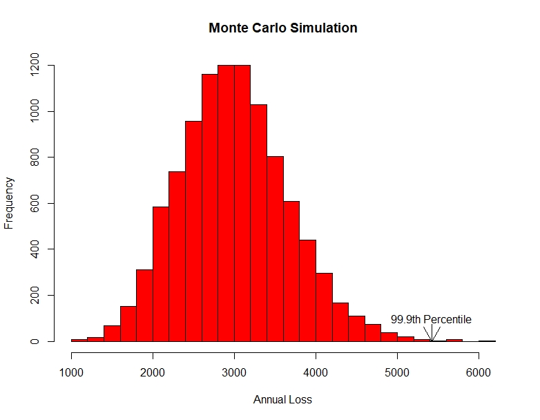
It is helpful to plot the resulting histogram of the 10,000 simulations. The real-world purpose of the exercise may be to identify the 99.9th percentile value. The R quantile function quantile(x, probs) returns the percentile value equal to probs. To display the percentile value on a plot, use the text and arrow functions. R has a text function that adds text a plot, text(x, y, label), which adds a label at coordinate (x,y). Further, R has an arrows function, arrows(x0, y0, x1, y1, code=2), which draws an arrow from (x0, y0) to (x1, y1) with code 2 drawing the arrowhead at (x1, y1).
The following is the R code and resulting histogram plot of a negative binomial frequency and lognormal severity simulation. The user input values are based on the mean and standard deviation values of a dataset.
# Monte Carlo simulation. Negative binomial frequency, lognormal severity.
# negbinom
nb_m <- 50 # This is a user input.
nb_sd <- 10 # This is a user input.
nb_var <- nb_sd^2
nb_size <- nb_m^2/(nb_var – nb_m)
# lognorm
xbar <- 60 # This is a user input.
sd <- 40 # This is a user input.
l_mean <- log(xbar) – .5*log((sd/xbar)^2 + 1)
l_sd <- sqrt(log((sd/xbar)^2 + 1))
num_sims <- 10000 # This is a user input.
set.seed(1234) # This is a user input.
rtotal <- vector()
for (i in 1:num_sims)
{
nb_random <- rnbinom(n=1, mu=nb_m, size=nb_size)
l_random <- rlnorm(nb_random, meanlog=l_mean, sdlog=l_sd)
rtotal[i] <- sum(l_random)
rtotal <- sort(rtotal)
m <- round(mean(rtotal), digits=0)
percentile_999 <- round(quantile(rtotal, probs=.999), digits=0)
print(paste(“Mean = “, m, ” 99.9th percentile = “, percentile_999))
hist(rtotal, breaks=20, col=”red”, xlab=”Annual Loss”, ylab=”Frequency”,
main=”Monte Carlo Simulation”)
text(percentile_999, 100, “99.9th Percentile”)
arrows(percentile_999,75, percentile_999,0, code=2)