How do I count thee? Let me count the ways?

How easily can you be identified on the Internet?

How easily can you be identified on the Internet? Suppose you finish your meal at a restaurant, you are about to pay the check, and t...

Friday, April 7, 2023

A more interesting pictorial numerical puzzle

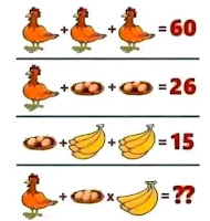
I am getting tired of these little pictorial numerical puzzles with the four equations, like one where three chickens equals 60, one chicken plus two plates of two eggs per plate equals 26, and so on, until the final equation is to evaluate some mathematical expression involving chickens, eggs, and bananas.

The solution generally requires that you remember the PEMDAS (in the US, or BODMAS elsewhere) rules for order of operations especially that multiplication takes precedence over addition, and also that you carefully count the number of eggs and number of bananas. I get 36.

OK, let me try to create a more interesting pictorial puzzle.

Mathematicians agree on the PEMDAS rules, although there are many situations that PEMDAS doesn't handle. Perhaps the most common is the unary minus operator as in -32. It is unary because unlike subtraction that has two operands, the unary operator only has one. I think mathematicians would like to see the unary operator as changing the sign of the argument, so that -32 equals -9, although some software, most notably Excel, merrily calculate this as +9.

I don't believe there is a single authority for all the order of operations cases. For example, Excel, Google Search, and Wolfram Alpha do not always agree. I bet there are some pretty smart people in those companies.

Nowadays I am doing my fun calculations in the R computer language, so for the remainder of this post I will require R as the authority.

So here is my attempt at a more interesting problem, but remember, you have to use the order of operation precedence rules of R: (Let me add the link to the first item: https://www.facebook.com/watch/?v=10158293605695705 )

Do you want to try it before I reveal the R code?


The R code is:

apple <- 1
banana <- 2
kiwi <- 3
lemon <- 4
peach <- banana + lemon
pear <- banana^banana^kiwi     # 2^(2^3) = 256
pineapple <- (pear - banana) %% kiwi^2 * lemon     # (254 %% 9) * 4 = 2 * 4 = 8
strawberry <- pineapple / peach * peach     # 8; no obelus in R
kiwi <- c(lemon, pineapple, strawberry)
watermelon <- kiwi[kiwi == lemon | kiwi == pineapple & kiwi == strawberry]
# watermelon <- (lemon V pineapple ∧ strawberry)     # 4 V (8 & 8) = 4, 8

The ordering rules of R include:

  • Modular arithmetic is at the same level as multiplication:     a mod b * c is     (a mod b) *c
  • The obelus does not appear in R but is just a division symbol:     a ÷ b * c = (a / b) * c
  • Repeated exponentiation goes right to left: a ^ b ^ c = a^(b^c); lots of disagreement outside R on this one
  • Logical AND preceds logical OR

Monday, March 27, 2023

There's a black hole in the number line

The government doesn't want you to know about this, but I have discovered it and I will share this with a few close friends: There is a black hole in the number line, and it's at number 4. Every word in the English language will eventually fall into it and can't get out of it.

As an example, take the word mathematical.

Mathematical has twelve letters.
Twelve has six letters.
Six has three letters.
Three has five letters.
Five has four letters.
Four has four letters.
Four has four letters, and now we entered this black hole at 4, and we can't get out of it!

Try a few more words. Try words as long as you like. Try morphophonemically, which has 18 letters. I have done exhaustive research on this with R, and you will find every English word eventually falls into the black hole at 4 and can't get out. At this rate, there will be no words left!

Of course, this is an April Fool's Day prank.

Did you figure it out?

Here is some R code to test the word mathematical.

# Try word mathematical
library(broman)
x <- "mathematical"
y <- -99 # Initialize y
while(y != "four"){
y <- nchar(x)
y <- broman::spell_out(y, max_value = 20) # Spell out an integer as a word
print(c(x,y))
x <- y
}

Here is some R code to test ten random words.

# Try ten random words
set.seed(123)
words <- read.table("https://raw.githubusercontent.com/dwyl/english-words/master/words_alpha.txt")
original <- sample(words$V1, 10, replace = FALSE)
x <- original
rm(words) # free up memory
for (i in 1:10){
y <- vector()
y[1] <- "dummy"
for (j in 1:100){
c <- nchar(x[i])
y[j] <- spell_out(c, max_value = 20)
x[i] <- y[j]
if (y[j] == "four") {
break
}
}
cat(c(original[i], "\t", y), "\n")
}

Here is the code for the number line:

library(ggplot2)
df <- data.frame(x = c(1,2,3,4,5,6,7,8,9,10),
y = rep(0,10),
group = c("A","A","A","B","A","A","A","A","A","A"))
ggplot(df, aes(x = x, y = y)) +
geom_point(aes(color = group, size = ifelse(x == 4, 15, 15))) +
geom_hline(yintercept = 0, linetype = 1, color = "lightblue", size = 1) +
scale_x_continuous(limits = c(0, 11), expand = c(0, 0),
breaks = NULL, minor_breaks = NULL) +
scale_y_continuous(limits = c(-0.2, 0.2), expand = c(0, 0),
breaks = NULL, minor_breaks = NULL) +
scale_color_manual(values = c("red", "black")) +
ggtitle("THE BLACK HOLE AT NUMBER 4") +
theme_void() +
theme(legend.position = "none",
axis.line = element_blank(),
axis.text = element_blank(),
plot.title = element_text(color="black", size=14, face="bold")) +
geom_text(aes(x = x, y = -0.1, label = x), size = 5)

Saturday, February 25, 2023

These drinking glasses are too short!

These drinking glasses are too short!

Some of my reinsurance and math teacher friends may remember that when I am out of town and having an adult beverage with friends, I have been known to stare at the drinking glass and say something like, "I don't mean to be rude, but the glasses are certainly short here. They are much shorter than what we have back home. In fact, they are so short, that I think that the circumference of the top of the glass is larger than the height."

Then there is generally a long pause as the group considers this. The reinsurance group may require some reminder of what circumference means.

Either group (unless they have heard this before, or unless they can guess that this is a setup) will likely disagree with me. I will reply that I am pretty sure about this, and I am willing to bet a dollar.

How do you measure this in a bar or restaurant? I use a paper or cloth napkin to measure the circumference from one end of the napkin to somewhere in the middle of the napkin, and then I use that length to compare to the height.

I have done this enough times so that I am nearly always right. Try it with your own drinking glasses. The only time it consistently fails is with champagne glasses.

Recently it occurred to me that there must be a website with a wide variety of glasses and their measurements, and I found Dimensions.com, https://www.dimensions.com . Dimensions.com is a database of drawings with standard measurements. Measurements are based on industry standards and averages and may differ among manufacturers and regions. Here is a sample of glasses with their images and measurements which are used here with permission, plus my calculations in the last three columns of the table. Volumes are in ounces, heights and diameters are in centimeters. The source is https://www.dimensions.com/collection/drinking-glasses and https://www.dimensions.com/collection/wine-glasses.

Here is some R code to do the calculations and to draw the above graph. Note that pi (lower case) is an inbuilt R constant whose value is approximately 3.141593. (Yes, I am well aware that π is an infinite, non-repeating decimal, and I believe R carries 16 decimal digits, but that is beyond the scope of this article.)

df <- data.frame(glass = c("Kalina10", "Pokal22", "Chardonnay", "XL Oversized","Cordial", "Shooter", "Champagne"),
volume = c(10, 22, 12.3, 25.36, 1.5, 2, 9),
height = c(11, 17.75, 19.8, 22.9, 15.9, 10.5, 23.5),
diameter = c(8, 9.5, 7.9, 10.8, 5.1, 4.13, 6.35))
df$circumference <- round(pi * df$diameter, 1)
df$larger <- ifelse(df$circumference > df$height, "Circumference", "Height")
df$c_to_h <- round(df$circumference / df$height, 1)
df

library(ggplot2)
ggplot(df, aes(x=factor(glass, level = c("Kalina10", "Pokal22", "Chardonnay", "XL Oversize","Cordial", "Shooter", "Champagne")), y=c_to_h, fill = glass, color="black")) +
geom_col(width = 1, position = position_dodge(1)) +
geom_hline(yintercept=1) +
ggtitle("Ratio of Circumference to Height by Glass") + xlab("Glass") + ylab("Ratio") +
theme(plot.title = element_text(face="bold", size=12)) +
theme(axis.text.x = element_text(face="bold", size=12)) +
theme(axis.text.y = element_text(size=12, face="bold")) +
theme(legend.position="none") +
scale_fill_manual("glass", values=c("red", "yellow", "blue", "green", "grey", "brown", "violet"))

I think the reason this is a good bet is that the mind can not easily compare a circular length to a linear length (I don't know if that is scientifically accurate), plus perhaps we look at the diameter but we forget we are comparing the height not to the diameter, but rather to π times the diameter.

Feel free to make this bet with your friends or your students. How about sharing 10% of your winnings with me as a commission?

Incidentally, a beverage can is approximately a right circular cylinder. (But not exactly; look at the top and bottom to see why.) Calculus students can derive that the cylinder with the largest volume for a given surface area (the surface area can be thought of as the rectangular area of the paper label around the entire can), has height equal to diameter. A typical 12 ounce soda can does not have height equal to diameter, but its circumference is greater than its height. A fun supermarket experiment is to examine different shaped cans (a soup can, a tuna fish can, etc.) to determine which meet the largest volume criterion.

To my reinsurance friends: I learned the circumference greater than height trick from Paul Hawksworth of M&G.

Sunday, February 12, 2023

Some different graph types in R

I don't know about you, but I get tired of seeing column charts and pie charts. It's not difficult to create a few more interesting chart types once in a while. Whether these are relevant for a particular audience and truly display your message is a different question.

I wanted a really small dataset to experiment in R, so I used numbers of days in office for US presidents who were assassinated. Students of American history may want to pause reading this post and think about whether you can name the Presidents (and estimate the number of days), before continuing reading. Kennedy and Lincoln are most well-known, but there were others.

I decided I wanted a column chart with images on the x-axis, a wordcloud with the font size proportional to the number of days, a lolliplot chart which is a variation of a column chart but with a line instead of a bar and a dot at the end, and a donut chart which is a variation of a pie chart but where your eye focuses on the length of the arc rather than on the area of the sector.

The first chart requires images. I grabbed the images I needed (hopefully these are either old or Federal and therefore not subject to copyright prohibitions) and saved them as png files so they could be read with a readPNG from the png package.

Of course there are many more chart types that are beyond the scope of this blog post. One reference is Top 50 ggplot2 Visualizations - The Master List (With Full R Code). A very cool chart type is the radar chart which you can see at How to Create Radar Charts in R (With Examples).

Here is my output (click to enlarge) and my R code:


setwd("C:/Users/ ... ")
suppressMessages(library(dplyr))
suppressMessages(library(ggplot2))
library(png)
library(ggtext)
df <- data.frame(President = c("Lincoln", "Garfield", "McKinley", "Kennedy"), Days_in_office = c(1503,199,1654,1036) )
# column chart with images on x-axis
p <- df %>%

ggplot() +
geom_col(mapping=aes(President, y=Days_in_office, fill=President)) +
scale_fill_manual(values=c("blue", "yellow", "red", "black")) +
labs(title="Axis Labels as Images") +
theme(plot.title = element_text(hjust = .5))

garfield <- readPNG("garfield.png")
kennedy <- readPNG("kennedy.png")
lincoln <- readPNG("lincoln.png")
mckinley <- readPNG("mckinley.png")
# in the following labels statement, please replace q with <, and replace z with >

labels <- c("qimg src='garfield.png', width='35' /z","qimg src='kennedy.png', width='35' /z","qimg src='lincoln.png', width='35' /z","qimg src='mckinley.png', width='40', height='42' /z")

p <- p +
scale_x_discrete(labels = labels) +
theme(axis.text.x = ggtext::element_markdown())
p # takes a moment to draw

# ==============================================================
suppressMessages(library(wordcloud))
df %>% with(wordcloud(words=President, freq=Days_in_office, random.order=FALSE, random.color=FALSE, rot.per = 0,
colors = c("blue","black", "red")))

# =====================================================
# lolliplot plot
df %>%
ggplot() +
geom_segment(mapping=aes(x=President, xend=President, y=0, yend=Days_in_office), color=c("blue", "yellow", "red", "black") ) +
geom_point(aes(x=President, y=Days_in_office), size=4, color=c("blue", "yellow", "red", "black") ) +
ylab("Days_in_office") +
theme(axis.text = element_text(face="bold")) +
theme(text = element_text(size =16)) +
labs(title="Lolliplot Plot") +
theme(plot.title = element_text(hjust = .5))
df

# ===========================================================
# donut plot
donut <- br="" df=""> donut$fraction = donut$Days_in_office / sum(donut$Days_in_office)

# Compute the cumulative percentages (top of each rectangle)
donut$ymax = cumsum(donut$fraction)

# Compute the bottom of each rectangle
donut$ymin = c(0, head(donut$ymax, n=-1))

# Compute label position

donut$labelPosition <- 2="" br="" donut="" ymax="" ymin="">

# Create label
donut$label <- ays_in_office="" br="" donut="" n="" paste0="" resident="" value:="">

# Make the plot
ggplot(donut, aes(ymax=ymax, ymin=ymin, xmax=4, xmin=3, fill=President)) +
geom_rect() +
geom_label( x=3.5, aes(y=labelPosition, label=label), size=6) +
scale_fill_brewer(palette=4) +
coord_polar(theta="y") +
xlim(c(2, 4)) +
theme_void() +
theme(legend.position = "none") +
theme(text = element_text(size =16)) +
labs(title="Donut Plot") +
theme(plot.title = element_text(hjust = .5))

Saturday, October 29, 2022

Find the next number in the sequence

Between ages two and four, most children can count up to at least ten.

If you ask your child, "What number comes next after 1, 2, 3, 4, 5?" they will probably say "6."

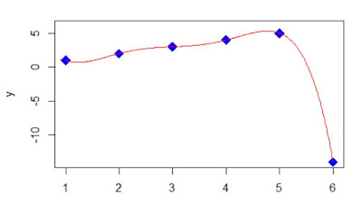
But to math nerds, any number can be the next number in a finite sequence. I like -14.

Given a sequence of n real numbers f(x1), f(x2), f(x3), ... , f(xn), there is always a mathematical procedure to find the next number f(x n+1) of the sequence. The resulting solution may not appear to be satisfying to students, but it is mathematically logical.

I can draw a smooth curve through the points (1,1), (2,2), (3,3), (4,4), (5,5), (6, -14). If I can find an equation for that smooth curve, then I know my answer of -14 has some logic to it. Actually many equations will work.

In my example one equation is of the form y = (x-1)*(x-2)*(x-3)*(x-4)*(x-5)*(A/120) + x, where A is chosen so that when x is 6, the first term reduces to A, and A + 6 equals the -14 I want. So A is -20. This is called a collocation polynomial.

There is a theorem that for n+1 distinct values of xi and their corresponding yi values, there is a unique polynomial P of degree n with P(xi) = yi. One method to find P is to use polynomial regression. Another way is to use Newton's Forward Difference Formula (probably no longer taught in Numerical Analysis courses).

Higher degree polynomials than degree n is one reason why additional equations will work.

The equation does not have to be a polynomial, which then adds rational functions among others.

Of course the next number after -14 can be any number. It could be 7 :)

There are many famous sequences, and of course someone catalogued them.

Here is some R code.

xpoints <- c(1,2,3,4,5,6)
ypoints <- c(1,2,3,4,5,-14)
y <- vector()
x <- seq(from=1, to=6, by=.01)
y <- (x-1)*(x-2)*(x-3)*(x-4)*(x-5)*(-20/120) + x
plot(xpoints, ypoints, pch=18, type="p", cex=2, col="blue", xlim=c(1,6), ylim=c(-14,6), xlab="x", ylab="y")
lines(x,y, pch = 19, cex=1.3, col = "red")
fit <- lm(ypoints ~ xpoints + I(xpoints^2) + I(xpoints^3) +I(xpoints^4) +I(xpoints^5) )
s <- summary(fit)
bo <- s$coefficient[1]
b1 <- s$coefficient[2]
b2 <- s$coefficient[3]
b3 <- s$coefficient[4]
b4 <- s$coefficient[5]
b5 <- s$coefficient[6]
x <- seq(from=1, to=6, by=.01)
z <- bo+b1*x+b2*x^2+b3*x^3+b4*x^4+b5*x^5
plot(xpoints, ypoints, pch=18, type="p", cex=2, col="blue", xlim=c(1,6), ylim=c(-14,6), xlab="x", ylab="y")
lines(x,z, pch = 19, cex=1.3, col = "red")

More great R blogs at r-bloggers.com

Saturday, September 17, 2022

How do I count thee? Let me count the ways?

by Jerry Tuttle   

In Major League Baseball, a player who hits 50 home runs in a single season has hit a lot of home runs. Suppose I want to count the number of 50 homer seasons by team, and also the number of 50 homer seasons by New York Yankees. (I will count Maris and Mantle in 1961 as two.) Here is the data including Aaron Judge's 62 in 2022 :

You would think base R would have a count function such as count(df$Team) and count(df$Team == "NYY") but this gives the error "could not find function 'count'". Base R does not have a count function.

Base R has at last four ways to perform a count:

1. The table function will count items in a vector.    table(df$Team) presents results horizontally, and data.frame(table(df$Team)) presents results vertically.    table(df$Team == "NYY") displays results 37 false and 10 true, while table(df$Team == "NYY")[2] just displays the result 10 true.

2. The sum function can be used to count the number of rows meeting a condition.    sum(df$Team == "NYY") displays the result 10. Here df$Team == "NYY" is creating a logical vector, and sum is summing the number of true = 1.

3. Similar to sum, nrow(df[df$Team == "NYY", ]) counts the number of rows meeting the NYY condition.

4. The length function counts the number of elements in an R object.    length(which(df$Team == "NYY")) , length(df$Team[df$Team == "NYY"]) , and length(grep("NYY", df[ , "Team"])) are all ways that will count the 10 Yankees.

The more direct solution to counting uses the count function in the dplyr library. Note that dplyr's count function applies to a data frame or tibble, but not to a vector. After loading library(dplyr) ,

1. df %>% count(Team) lists the count for each team.

2. df %>% filter(Team = "NYY") lists each Yankee, and you can see there are 10.

3. df %>% count(Team == "NYY") displays 37 false and 10 true, while df %>% filter(Team == "NYY") %>% count() just displays the 10 true.

The following is a bar chart of the results by team for teams with at least 1 50 homer season:

Finally, "How do I count thee? Let me count the ways?" is of course adapted from Elizabeth Barrett Browning's poem "How do I love thee? Let me count the ways?" But in her poem, just how would we count the number of times "love" is mentioned? The tidytext library makes counting words fairly easy, and the answer is ten, the same number of 50 homer Yankee seasons. Coincidence?

The following is all the R code. Happy counting!

library(dplyr)
library(ggplot2)
library(tidytext)

df <- data.frame(
   Player=c('Ruth','Ruth','Ruth','Ruth','Wilson','Foxx','Greenberg','Foxx','Kiner','Mize','Kiner','Mays','Mantle','Maris', 'Mantle','Mays','Foster','Fielder','Belle','McGwire','Anderson','McGwire','Griffey','McGwire','Sosa','Griffey', 'Vaughn','McGwire','Sosa','Sosa','Bonds','Sosa','Gonzalez','Rodriguez','Rodriguez','Thome','Jones','Howard','Ortiz', 'Rodriguez','Fielder','Bautista','Davis','Stanton','Judge','Alonso','Judge'),
   Year=c(1920,1921,1927,1928,1930,1932,1938,1938,1947,1947,1949,1955,1956,1961,1961,1965,1977,1990,1995,1996,1996,1997,1997, 1998,1998,1998,1998,1999,1999,2000,2001,2001,2001,2001,2002,2002,2005,2006,2006,2007,2007,2010,2013,2017,2017,2019,2022),
   Homers=c(54,59,60,54,56,58,58,50,51,51,54,51,52,61,54,52,52,51,50,52,50,58,56,70,66,56,50,65,63,50,73,64,57,52,57,52,51, 58,54,54,50,54,53,59,52,53,62),
   Team=c('NYY','NYY','NYY','NYY','CHC','PHA','DET','BOS','PIT','NYG','PIT','NYG','NYY','NYY','NYY','SF','CIN','DET','CLE', 'OAK','BAL','OAK/SLC','SEA','SLC','CHC','SEA','SD','SLC','CHC','CHC','SF','CHC','ARI','TEX','TEX','CLE','ATL','PHP', 'BOR','NYY','MIL','TOR','BAL','MIA','NYY','NYM','NYY'))

head(df)

# base R ways to count:

table(df$Team)    # shows results horizontally
data.frame(table(df$Team))    #shows results vertically
table(df$Team == "NYY")    # displays 37 false and 10 true
table(df$Team == "NYY")[2]

sum(df$Team == "NYY")    # displays the result 10.

nrow(df[df$Team == "NYY", ])    # counts the number of rows meeting the NYY condition.

length(which(df$Team == "NYY"))     # which returns a vector of indices which are true
length(df$Team[df$Team == "NYY"])
length(grep("NYY", df[ , "Team"]))     # grep returns a vector of indices that match the pattern

# dplyr R ways to count; remember to load library(dplyr):

df %>% count(Team)    # lists the count for each team.

df %>% filter(Team == "NYY")    # lists each Yankee, and you can see there are 10.

df %>% count(Team == "NYY")    # displays 37 false and 10 true, while
df %>% filter(Team == "NYY") %>% count()    # just displays the 10 true.

# barplot of all teams with at least 1 50 homer season; remember to load library(ggplot2)

df %>%
    group_by(Team) %>%
    summarise(count = n()) %>%
    ggplot(aes(x=reorder(Team, count), y=count, fill=Team)) +
    geom_bar(stat = 'identity') +
    ggtitle("Count of 50 Homer Seasons") +
    xlab("Team") +
    scale_y_continuous(breaks=c(1,2,3,4,5,6,7,8,9,10)) +
    coord_flip() +
    theme(plot.title = element_text(face="bold", size=18)) +
    theme(axis.title.y = element_text(face="bold")) +
    theme(axis.title.x = element_blank()) +
    theme(axis.text.x = element_text(size=12, face="bold"),
    axis.text.y = element_text(size=12, face="bold")) +
    theme(legend.position="none")

# count number of times "love" is mentioned in Browning's poem; remember to load library(tidytext)

textfile <- c("How do I love thee? Let me count the ways.",
"I love thee to the depth and breadth and height",
"My soul can reach, when feeling out of sight",
"For the ends of being and ideal grace.",
"I love thee to the level of every day's",
"Most quiet need, by sun and candle-light.",
"I love thee freely, as men strive for right.",
"I love thee purely, as they turn from praise.",
"I love thee with the passion put to use",
"In my old griefs, and with my childhood's faith.",
"I love thee with a love I seemed to lose",
"With my lost saints. I love thee with the breath,",
"Smiles, tears, of all my life; and, if God choose,",
"I shall but love thee better after death.")

df<-data.frame(line=1:length(textfile), text=textfile)
df_words <- df %>% unnest_tokens(word, text)
cleaned_words <- df_words %>% anti_join(get_stopwords())
cleaned_words %>% count(word, sort = TRUE) %>% head(6)
cleaned_words %>% filter(word == "love") %>% count()

More great R blogs at r-bloggers.com

Wednesday, June 22, 2022

What is the difference between statistics and data analysis?

What is the difference between statistics and data analysis?

Of course to answer this we need to define those terms, and definitions of such things are hardly standard. But they are nor particularly standard in other disciplines either. Can you define art? Music? How about mathematics?

Would you have defined mathematics as "including such topics as numbers, formulas and related structures, shapes and the spaces in which they are contained, and quantities and their changes," as in Wikipedia? Is this all-encompassing?

Statistics and data analysis have some overlaps. Both involve defining, exploring, cleaning, visualizing, and describing data. Data analyst students study some traditional statistics. Statistics students nowadays study some data analysis.

The father and daughter Larose team have suggested a working distinction of inferential statistics versus data mining (so neither of these is identical to the terms in the first sentence above) as follows:

Inferential statistics involves having a prior hypothesis about a population and testing that hypothesis with a sample from that population. The test may result in statistical significance, even if there is no practical significance.

Data mining does not begin with a prior hypothesis, but rather the analyst "freely trolls through the data for actionable results." (Larose, p. 161)

Larose, D.T. & Larose, C.D. (2015). Data mining and predictive analytics. Wiley. Hoboken, NJ.